Last updated on August 12th 2016.

Note

The following links shows the example project as it should be just before step 13. You can use this to check your progress or restart the tutorial at this very point.

After Step 13: Synthetics

14. Misfit and Adjoint Source Calculation

In order to calculate sensitivity kernels (gradients) for a given combination of model and data, one needs calculate the adjoint sources. An adjoint source is usually dependent on the misfit between the synthetics and real data.

LASIF currently supports misfits in the time-frequency domain as defined by Fichtner et al. (GJI 2008) Great care has to be taken to avoid cycle skips/phase jumps between synthetics and data. This is achieved by careful windowing.

14.1. Weighting Scheme

You may notice that at various points it is possible to distribute weights. These weights all contribute to the final adjoint source. The inversion scheme requires one adjoint source per iteration, event, station, and component.

In each iteration’s XML file you can specify the weight for each event, denoted as \(w_{event}\) and within each event, the weight per station \(w_{station}\). Both weights are allowed to range between 0.0 and 1.0. A weight of 0.0 corresponds to no weight at all, e.g. skip the event and a weight of 1.0 is the maximum weight.

<?xml version='1.0' encoding='UTF-8'?>
<iteration>
  <iteration_name>1</iteration_name>
  ...
  <event>
    <event_name>GCMT_event_NORTHWESTERN_BALKAN_REGION_Mag_5.9_1980-5-18-20-2</event_name>
    <event_weight>1.0</event_weight>
    <station>
      <station_id>LA.AA22</station_id>
      <station_weight>1.0</station_weight>
    </station>
    <station>
      ...
    </station>
  </event>
    ...
  <event>
  </event>
</iteration>

You can furthermore choose an arbitrary number of windows per component for which the misfit and adjoint source will be calculated. Each window has a separate weight, with the only limitation being that the weight has to be positive. These weights can be edited after the windows have been selected.

Assuming \(N\) windows in a given component, the corresponding adjoint sources will be called \(adj\_source_{1..N}\) while their weights are \(w_{1..N}\). The final adjoint source for every component will be calculated according to the following formula:

\[adj\_source = w_{event} \cdot w_{station} \cdot \frac{1}{\sum_{i=1}^N w_i} \cdot \sum_{i=1}^N w_i \cdot ad\_src_i\]

14.2. Misfit GUI

LASIF comes with a graphical utility called the Misfit GUI, that helps to pick correct windows. To launch it, simply type

$ lasif launch_misfit_gui

This will open a window that looks like the following:

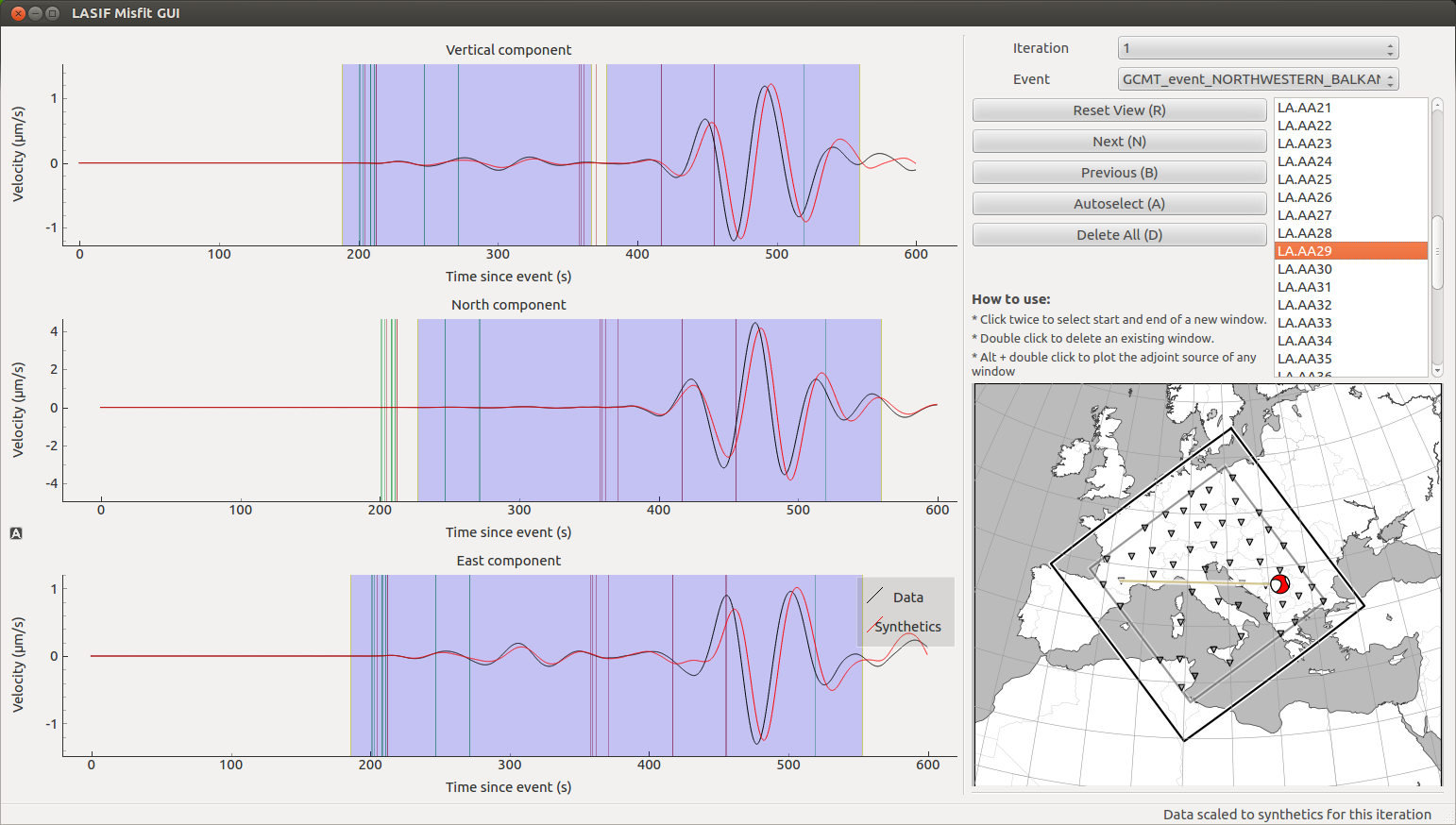
In the top right part of the GUI, you can choose which iteration and which event you want to see the synthetics of. The scroll menu shows all the stations for which data are available, and you can go to the next station using either mouse or keyboard up/down arrows. The map in the bottom right will show which event-station combination is currently plotted.

With the Next and Prev button you can jump from one station to the next. The Delete All button will remove all windows for the current station. Autoselect will run the automatic window selection algorithm for the currently selected station.

To actually choose a window click twice - once for the start and once for the end of a window. It will be saved and the adjoint source will be calculated.

Double clicking on an already existing window will delete it, Alt + clicking will show the time frequency phase misfit as well as the calculated adjoint source.

The windows are saved in the window XML files (saved on a per-station basis in the ADJOINT_SOURCES_AND_WINDOWS/WINDOWS/{{EVENT_NAME}}/ITERATION_{{ITERATION_NAME}}/ folder), and currently, this is the only place where the window weights can be adjusted.

14.3. Window Selection

As an alternative to going through each event-station pair, you can tell LASIF to select the windows automatically using

$ lasif select_windows 1 GCMT_event_NORTHWESTERN_BALKAN_REGION_Mag_5.9_1980-5-18-20-2

for a single event in iteration 1, or

$ lasif select_all_windows

for all events in the iteration (the latter can also be run with mpirun -n X .... Use these tools with caution and check their result!

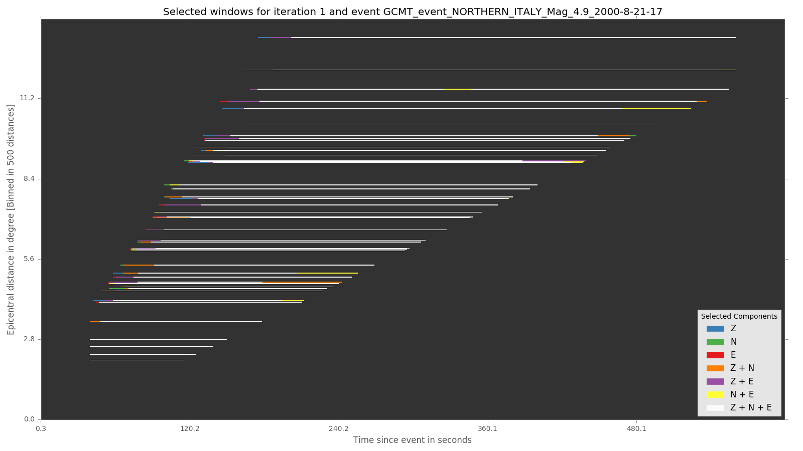
LASIF comes with a number of utilities to judge the quality of selected windows. One of these plots a summary of the temporal and epicentral distance distribution of selected events:

$ lasif plot_windows --combine 1 GCMT_event_NORTHERN_ITALY_Mag_4.9_2000-8-21-17

14.4. Final Adjoint Source Calculation

During window selection, the adjoint source for each chosen window will be stored separately. To combine them, apply the weighting scheme and convert them to a format, that SES3D can actually use, run the finalize_adjoint_sources command with the iteration name and the event name.

$ lasif finalize_adjoint_sources 1 GCMT_event_NORTHERN_ITALY_Mag_4.9_2000-8-21-17
$ lasif finalize_adjoint_sources 1 GCMT_event_NORTHWESTERN_BALKAN_REGION_Mag_5.9_1980-5-18-20

This will also rotate the adjoint sources to the frame of reference used in the simulations.

If you pick any more windows or change them in any way, you need to run the command again. The result of that command is a list of adjoint sources directly usable by SES3D in the OUTPUT folder.

Copy these to the correct folder inside your SES3D installation, make sure to tell SES3D to perform an adjoint reverse simulation and launch it. Please refer to the SES3D manual for the necessary details.

14.5. Gradient visualisation

It is possible to view the raw gradients from a SES3D simulation. To do this, simply put them, along with the boxfile that is used in SES3D, in the a folder according to the following scheme:

KERNELS/ITERATION_{{ITERATION_NAME}}/{{EVENT_NAME}}

For the example in the tutorial this results in the two folders:

• KERNELS/ITERATION_1/GCMT_event_NORTHERN_ITALY_Mag_4.9_2000-8-21-17-14
• KERNELS/ITERATION_1/GCMT_event_NORTHWESTERN_BALKAN_REGION_Mag_5.9_1980-5-18-20-2

If the folder inside an iteration has the name of an event it is assumed to be the gradient from that particular event. If it has any other name it can still be plotted but you have to take care of the meaning.

The plot_kernel command can be used to plot the gradients/kernels and usage is similar to the plot_events command. However, components are now called grad_{{COMPONENT}} – the same component names as the files you copied into the kernels folder. So to plot the gradient for SV velocity at 50 km depth for the first event, type

$ lasif plot_kernel KERNELS/ITERATION_1/GCMT_event_NORTHERN_ITALY_Mag_4.9_2000-8-21-17/ 50 grad_csv Kernel.050km.vsv.png

Note that the kernel for vsv is called grad_csv – likewise for the other velocities.

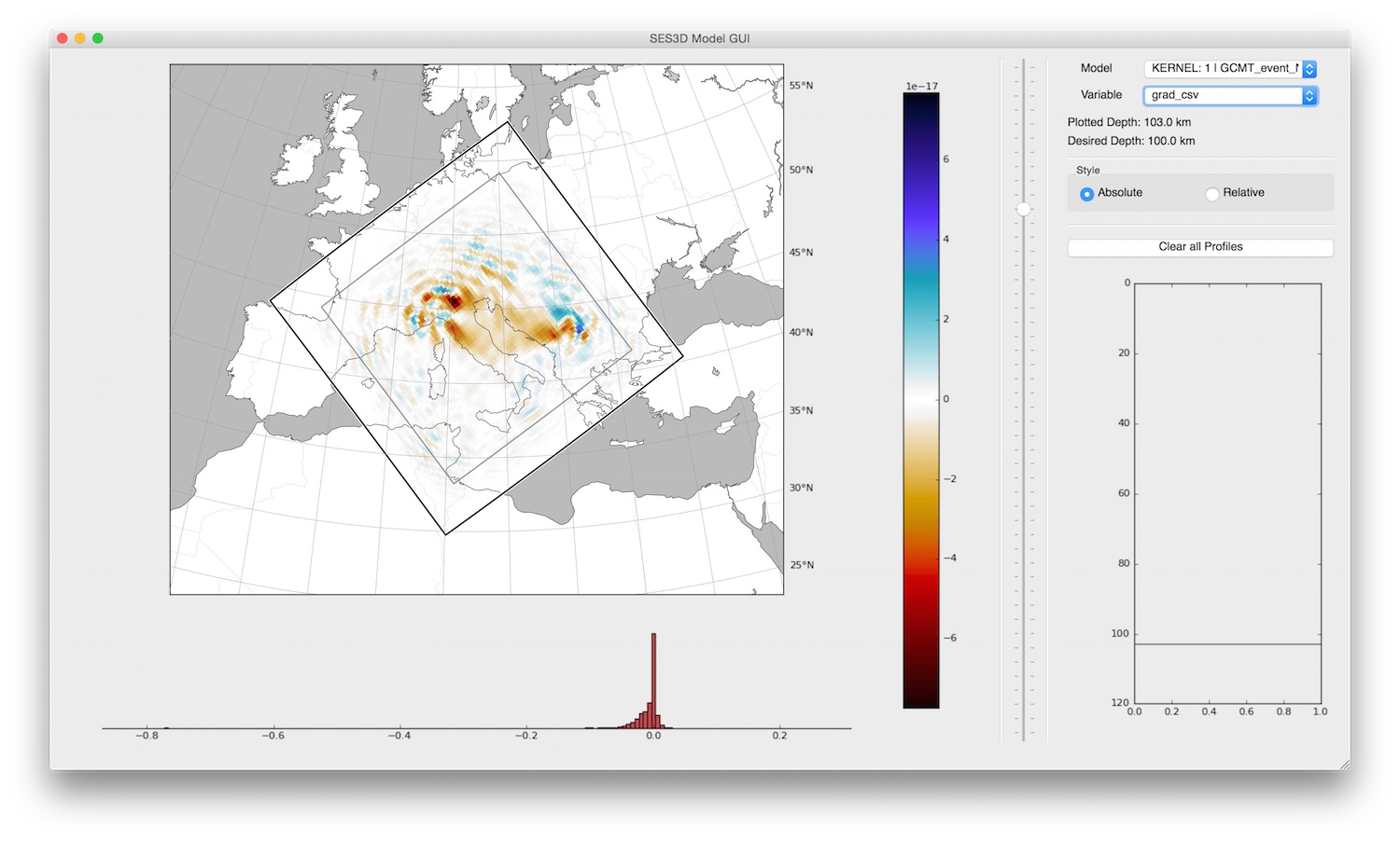
Alternatively, you can again use the model gui in order to explore the kernels. This works exactly the same as before, just select your favourite KERNEL: {{ITERATION_NAME}} | {{EVENT_NAME}}. If all is well, it looks like this for the raw, unsmoothed vsv kernel: