Last updated on August 12th 2016.
9. Defining a New Iteration
LASIF organizes the actual inversion in an arbitrary number of iterations; each of which is described by a single XML file. Within each file, the events and stations for this iterations, the solver settings, and other information is specified. Each iteration can have an arbitrary name. It is probably a good idea to give simple numeric names, like 1, 2, 3, …
Let’s start by creating the XML file for the first iteration with the
create_new_iteration command.
$ lasif create_new_iteration 1 40.0 100.0 SES3D_4_1

Starting to find optimal relaxation parameters.
weights:              [1.4171098866795313, 0.7083736187912052, 1.2711221163303799]
relaxation times:     [2.1698930654135467, 8.8998280969528185, 30.931200043682129]
partial derivatives:  [-2.03196917  0.04160294  2.85511248]
cumulative rms error: 0.0125298336474
This command takes four arguments; the first being the iteration name. A simple
number is sufficient in many cases. The second and third denote the band limit
of this iteration. In this example, the band is limited between 40 and 100
seconds. The fourth argument is the waveform solver to be used for this
iteration. It currently supports some versions of SES3D as well as the
cartesian and global versions of SPECFEM but the infrastructure to add other
solvers is already in place. See the help of the create_new_iteration
command to get a list of all supported solvers.
You will see that this creates a new file: ITERATIONS/ITERATION_1.xml.
Each iteration will have its own file. To get a list of iterations, use
$ lasif list_iterations

1 Iteration in project:
    1
To get more information about a specific iteration, use the iteration_info
command.
$ lasif iteration_info 1

LASIF Iteration
    Name: 1
    Description: None
    Preprocessing Settings:
        Highpass Period: 100.000 s
        Lowpass Period: 40.000 s
    Solver: SES3D 4.1 | 500 timesteps (dt: 0.75s)
    2 events recorded at 51 unique stations
    102 event-station pairs ("rays")
Note
You might have noticed the pairs of list_x and x_info commands, e.g.
list_events and event_info or list_iterations and
iteration_info. This scheme is true for most things in LASIF. The
list_x variant is always used to get a quick overview of everything
currently part of the LASIF project. The x_info counterpart returns
more detailed information about the resource.
Note
As mentioned before, it is entirely possible to add new events at a later
stage during an inversion. Be aware, however, that these events will only
show up in a subsequent iteration that is created using the
create_new_iteration command, because all events and stations used in
any given iteration are explicitly defined in the iteration xml file.
9.1. The Iteration XML Files
The XML file defining each iteration attempts to be a collection of all information relevant for a single iteration.
Note
The iteration XML files are the main provenance information (in combination with the log files) within LASIF. By keeping track of what happened during each iteration it is possible to reasonably judge how any model came into being.
If at any point you feel the need to keep track of additional information and there is no place for it within LASIF, please contact the developers. LASIF aims to offer an environment where all necessary information can be stored in an organized and sane manner.
The iteration XML files currently contain:
- Some metadata: the iteration name, a description and some comments.
- A limited data preprocessing configuration. The data preprocessing is currently mostly fixed and only the desired frequency content can be chosen. Keep in mind that these values will also be used to filter the source time function.
- The settings for the solver used for this iteration.
- A list of all events used for the iteration. Here it is possible to apply weights to the different events and also to apply a time correction. It can differ per iteration.
- Each event contains a list of stations where data is available. Furthermore each station can have a different weight and time correction.
Let’s have a quick look at the generated file. The create_new_iteration
command will create a new iteration file with all the information currently
present in the LASIF project.
<?xml version='1.0' encoding='UTF-8'?>
<iteration>
  <iteration_name>1</iteration_name>
  <iteration_description></iteration_description>
  <comment></comment>
  <scale_data_to_synthetics>true</scale_data_to_synthetics>
  <data_preprocessing>
    <highpass_period>100.0</highpass_period>
    <lowpass_period>40.0</lowpass_period>
  </data_preprocessing>
  <solver_parameters>
    <solver>SES3D 4.1</solver>
    <solver_settings>
      <simulation_parameters>
        <number_of_time_steps>2000</number_of_time_steps>
        <time_increment>0.3</time_increment>
        <is_dissipative>false</is_dissipative>
      </simulation_parameters>
      <output_directory>../OUTPUT/CHANGE_ME/{{EVENT_NAME}}</output_directory>
      <adjoint_output_parameters>
        <sampling_rate_of_forward_field>10</sampling_rate_of_forward_field>
        <forward_field_output_directory>../OUTPUT/CHANGE_ME/ADJOINT/{{EVENT_NAME}}</forward_field_output_directory>
      </adjoint_output_parameters>
      <computational_setup>
        <nx_global>24</nx_global>
        <ny_global>24</ny_global>
        <nz_global>15</nz_global>
        <lagrange_polynomial_degree>4</lagrange_polynomial_degree>
        <px_processors_in_theta_direction>2</px_processors_in_theta_direction>
        <py_processors_in_phi_direction>2</py_processors_in_phi_direction>
        <pz_processors_in_r_direction>1</pz_processors_in_r_direction>
      </computational_setup>
      <relaxation_parameter_list>
        ...
      </relaxation_parameter_list>
    </solver_settings>
  </solver_parameters>
  <event>
    <event_name>GCMT_event_NORTHWESTERN_BALKAN_REGION_Mag_5.9_1980-5-18-20</event_name>
    <event_weight>1.0</event_weight>
    <station>
      <station_id>LA.AA22</station_id>
      <station_weight>1.0</station_weight>
    </station>
    ...
  </event>
  ...
</iteration>
It is a rather self-explanatory file, but some things to look out for:
- The dataprocessing frequency limits are given periods in seconds. This is more in line with what one would normally use than frequencies in Hz.
- The paths in the solver settings contains an
{{EVENT_NAME}}part. This part will be replaced by the actual event name. This means that the file does not have to be adjusted for every event.
Note
The file shown here has already been adjusted for the tutorial example. For the tutorial we will run a simulation on 4 cores (should be suitable for your desktop PC/laptop) for 2000 timesteps with a time delta of 0.3 seconds. Please make sure to also adjust the file accordingly. The following parameters are essential in almost all cases (shown here with the values for the tutorial):
number_of_time_steps:2000time_increment:0.3is_dissipative:false(in a real world application set this totrue)nx_global:24ny_global:24nz_global:15px_processors_in_theta_direction:2py_processors_in_phi_direction:2pz_processors_in_r_direction:1
Please refer to the SES3D documentation for more information. The SES3D documentation can currently be obtained from the tarball found here (link most recently checked on 13 June 2016).
9.2. Source Time Functions
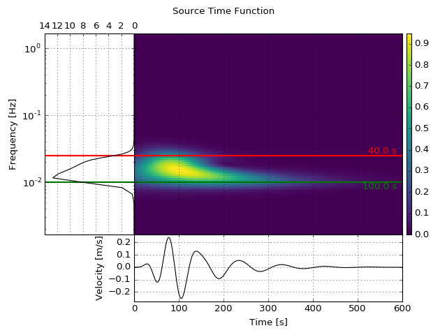
The source time functions will be generated dynamically from the information specified in the iteration XML files. Currently only one type of source time function, a filtered Heaviside function is supported. In the future, if desired, it could also become possible to use inverted source time functions.
The source time function will always be defined for the number of time steps and the time increment you specify in the solver settings. Furthermore, all source time functions will be filtered with the same bandpass as the data.
To have a quick look at the source time function for any given iteration, use
the plot_stf command with the iteration name:
$ lasif plot_stf 1
This command will read the corresponding iteration file and open a plot with a time series and a time frequency representation of the source time function.
(Source code, png, hires.png, pdf)

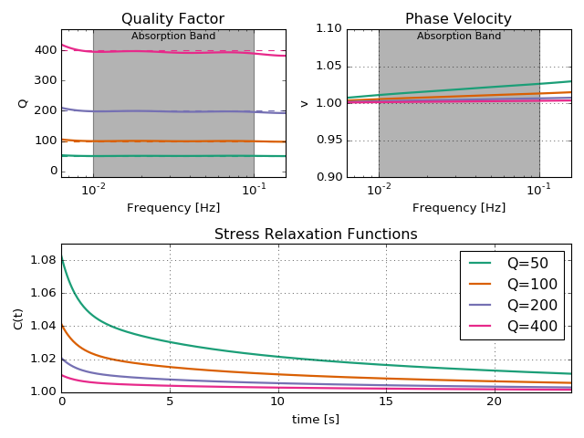
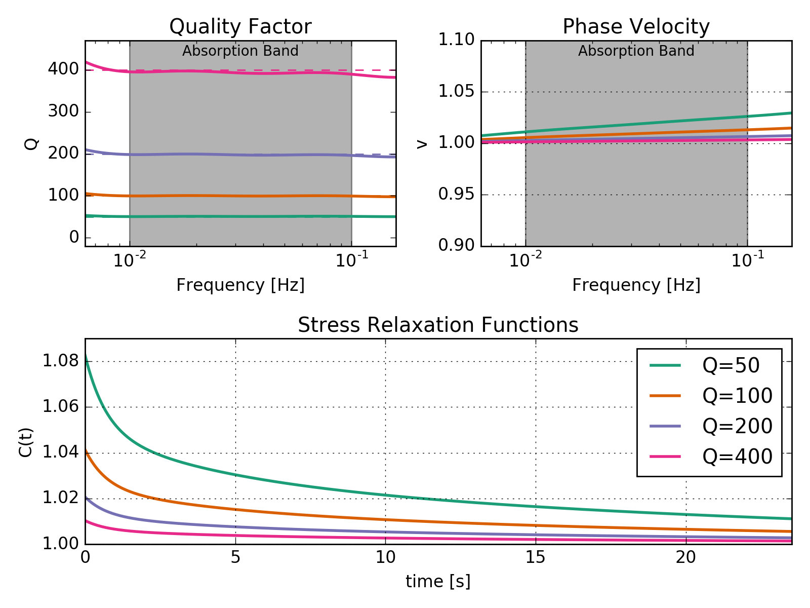
9.3. Attenuation
SES3D models attenuation with a discrete superposition of a finite number of relaxation mechanisms. The goal is to achieve a constant Q model over the chosen frequency range. Upon creating an iteration, LASIF will run a non-linear optimization algorithm to find relaxation times and associated weights that will be nearly constant over the chosen frequency domain.
At any point you can see the absorption-band model for a given iteration at a couple of exemplary Q values with
$ lasif plot_Q_model 1
The single argument is the name of the iteration.
(Source code, png, hires.png, pdf)

The grey band in each plot marks the frequency range as specified in the iteration XML file.
It is also possible to directly generate the relaxation times and weights for any frequency band. To generate a Q model that is approximately constant in a period band from 10 seconds to 100 seconds use
$ lasif calculate_constant_Q_model 40 100

Starting to find optimal relaxation parameters.
weights:              [1.4474, 0.7336, 1.2757]
relaxation times:     [2.0279, 8.7190, 31.0539]
partial derivatives:  [-2.0727 -0.0131  2.8965]
cumulative rms error: 0.01255