mtspec.wigner_ville_spectrum

mtspec.multitaper.wigner_ville_spectrum(data, delta, time_bandwidth=3.5, number_of_tapers=None, smoothing_filter=None, filter_width=100, frequency_divider=1, verbose=False)

Function to calculate the Wigner-Ville Distribution or Wigner-Ville Spectrum of a signal using multitaper spectral estimates.

In general it gives better temporal and frequency resolution than a spectrogram but introduces many artifacts and possibly negative values which are not physical. This can be alleviated a bit by applying a smoothing kernel which is also known as a reduced interference distribution (RID).

Wraps the wv_spec() and wv_spec_to_array() subroutines of the Fortran library.

It is very slow for large arrays so try with a small one (< 5000 samples) first.

Parameters:

• data (numpy.ndarray) – The input signal.
• delta (float) – The sampling interval of the data.
• time_bandwidth (float) – Time bandwidth product for the tapers.
• number_of_tapers (int) – Number of tapers to use. If None, the number will be automatically determined from the time bandwidth product which is usually the optimal choice.
• smoothing_filter (str) – One of "boxcar", "gauss" or just None
• filter_width (int) – Filter width in samples.
• frequency_divider (int) – This method will always calculate all frequencies from 0 … Nyquist frequency. This parameter allows the adjustment of the maximum frequency, so that the frequencies range from 0 .. Nyquist frequency / int(frequency_divider).
• verbose (bool) – Verbose output on/off.

Example

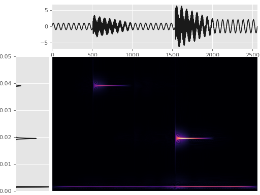
This example demonstrates how to plot a signal, its multitaper spectral estimate, and its Wigner-Ville time-frequency distribution. The signal is sinusoidal overlaid with two simple linear chirps.

>>> import matplotlib.pyplot as plt
>>> import numpy as np
>>> from mtspec import mtspec, wigner_ville_spectrum
>>> from mtspec.util import signal_bursts
>>> fig = plt.figure()

Get the example signal.

>>> data = signal_bursts()

Plot the data on the top axes.

>>> ax1 = fig.add_axes([0.2,0.75, 0.79, 0.23])
>>> ax1.plot(data, color="0.1")
>>> ax1.set_xlim(0, len(data))

Plot its spectral estimate on the side.

>>> ax2 = fig.add_axes([0.06,0.02,0.13,0.69])
>>> spec, freq = mtspec(data, 10, 3.5)
>>> ax2.plot(spec, freq, color="0.1")
>>> ax2.set_xlim(0, spec.max())
>>> ax2.set_ylim(freq[0], freq[-1])
>>> ax2.set_xticks([])

Create and plot the Wigner-Ville distribution.

>>> wv = wigner_ville_spectrum(data, 10, 3.5,
...                            smoothing_filter='gauss')
>>> ax3 = fig.add_axes([0.2, 0.02, 0.79, 0.69])
>>> ax3.set_yticks([])
>>> ax3.set_xticks([])
>>> # The square root only serves plotting purposes.
>>> ax3.imshow(np.sqrt(abs(wv)), interpolation='lanczos',
...            aspect='auto', cmap="magma")

(Source code, png, hires.png, pdf)