![]()
Exercise -- The 2008 Mt. Carmel, Illinois, Earthquake and Aftershock Series
Introduction from "The April 18, 2008 Illinois Earthquake: An ANSS Monitoring Success" by Robert B. Herrmann, Mitch Withers, and Harley Benz, SRL 2008:
"The largest-magnitude earthquake in the past 20 years struck near Mt. Carmel in southeastern Illinois on Friday morning, 18 April 2008 at 09:36:59 UTC (04:37 CDT). The Mw 5.2 earthquake was felt over an area that spanned Chicago and Atlanta, with about 40,000 reports submitted to the U.S. Geological Survey (USGS) “Did You Feel It?” system. There were at least six felt aftershocks greater than magnitude 3 and 20 aftershocks with magnitudes greater than 2 located by regional and national seismic networks. Portable instrumentation was deployed by researchers of the University of Memphis and Indiana University (the first portable station was installed at about 23:00 UTC on 18 April). The portable seismographs were deployed both to capture near-source, high-frequency ground motions for significant aftershocks and to better understand structure along the active fault. [...]"


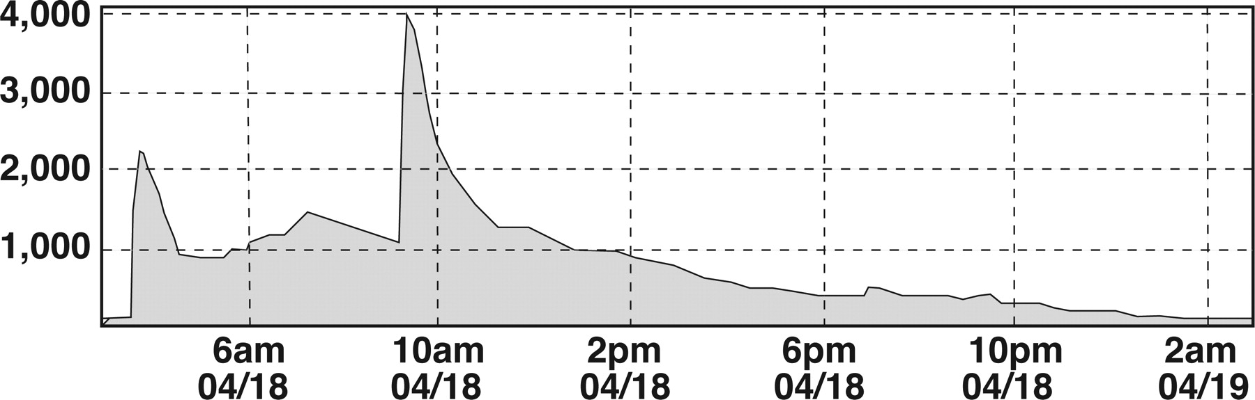
Web page hits at USGS/NEIC during 24 hours after the earthquake:
- peak rate: 3,892 hits/second
- 68 million hits in the 24 hours after the earthquake
Some links:
%matplotlib inline
Use the search on the ObsPy docs for any functionality that you do not remember/know yet..!
E.g. searching for "filter"...
1. Download and visualize main shock
Request information on stations recording close to the event from IRIS using the obspy.fdsn Client, print the requested station information.
Download waveform data for the mainshock for one of the stations using the FDSN client (if you get an error, maybe try a different station and/or ask for help). Make the preview plot using obspy.
Visualize a Spectrogram (if you got time, you can play around with the different parameters for the spectrogram). Working on a copy of the donwloaded data, apply a filter, then trim the requested data to some interesting parts of the earthquake and plot the data again.
Define a function plot_data(t) that fetches waveform data for this station and that shows a preview plot of 20 seconds of data starting at a given time. It should take a UTCDateTime object as the single argument.
Test your function by calling it for the time of the main shock
2. Visualize aftershock and estimate magnitude
Read file "./data/mtcarmel.mseed". It contains data of stations from an aftershock network that was set up shortly after the main shock. Print the stream information and have a look at the network/station information, channel names time span of the data etc.. Make a preview plot.
The strongest aftershock you see in the given recordings is at 2008-04-21T05:38:30. Trim the data to this aftershock and make a preview plot and a spectrogram plot of it.
Make a very simple approximation of the magnitude. Use the function provided below (after you execute the code box with the function you can call it anywhere in your code boxes).
Demean the data and then determine the raw data's peak value of the event at one of the stations (e.g. using Python's max function or a numpy method on the data array) and call the provided function for that value. (Note that this is usually done on the horizontal components.. we do it on vertical for simplicity here)
from obspy.signal.invsim import estimate_magnitude

def mag_approx(peak_value, frequency, hypo_dist=20):
    """
    Give peak value of raw data for a very crude and simple magnitude estimation.

    For simplicity, this is done assuming hypocentral location, peak frequency, etc.
    To keep it simple for now the response information is entered manually here
    (it is the same for all instruments used here).
    """
    poles = [-1.48600E-01  + 1.48600E-01j,
             -1.48600E-01  - 1.48600E-01j,
             -4.14690E+02  + 0.00000E+00j,
             -9.99027E+02  + 9.99027E+02j,
             -9.99027E+02  - 9.99027E+02j]
    zeros = [0.0 + 0.0j,
             0.0 + 0.0j,
             1.1875E+03 + 0.0j]
    norm_factor = 7.49898E+08
    sensitivity = 6.97095E+05
    paz = {'poles': poles, 'zeros': zeros, 'gain': norm_factor,
           'sensitivity': sensitivity}
    ml = estimate_magnitude(paz, peak_value, 0.5 / frequency, hypo_dist)
    return ml
Do the magnitude approximation in a for-loop for all stations in the Stream. Calculate a network magnitude as the average of all three stations.
Define a function netmag(st) that returns a network magnitude approximation. It should take a Stream object (which is assumed to be trimmed to an event) as only argument. Use the provided mag_approx function and calculate the mean of all traces in the stream internally.
Test your function on the cut out Stream object of the large aftershock from before.
Advanced
You can also download the station metadata using the FDSN client and extract poles and zeros information and directly use the estimate_magnitude function without using the hard-coded response information.
3. Detect aftershocks using triggering routines
Read the 3-station data from file "./data/mtcarmel.mseed" again. Apply a bandpass filter, adjust it to the dominant event frequency range you have seen in the aftershock spectrogram before. Run a recursive STA/LTA trigger on the filtered data (see ObsPy docs). The length of the sta window should be a bit longer than an arriving seismic phase, the lta window can be around ten to twenty times as long.
Make a preview plot of the Stream object, now showing the characteristic function of the triggering. High trigger values indicate transient signals (of the frequency range of interest) that might be an event (or just a local noise burst on that station..).
(play around with different values and check out the resulting characteristic function)
We could now manually compare trigger values on the different stations to find small aftershocks, termed a network coincidence trigger. However, there is a convenience function in ObsPy's signal toolbox to do just that in only a few lines of code.
Read the data again and apply a bandpass to the dominant frequencies of the events. Use the coincidence_trigger function that returns a list of possible events (see the ObsPy Tutorial for an example of a recursive STA/LTA network coincidence trigger). Print the length of the list and adjust the trigger-on/off thresholds so that you get around 5 suspected events.
Print the first trigger in the list to show information on the suspected event.
Go over the list of triggers in a for-loop. For each trigger/suspected event:
- print the time of the trigger
- read the waveform data, use
starttimeandendtimearguments forread()to trim the data to the suspected event right during reading (avoiding to read the whole file again and again) - calculate and print the network magnitude using the
netmag(st)function from earlier - make a preview plot
If you're curious you can compare the crude magnitude estimates with the table of aftershocks provided by the scientists that analyzed the aftershock sequence. The paper with details can be found here: "Aftershocks of the 2008 Mt. Carmel, Illinois, Earthquake: Evidence for Conjugate Faulting near the Termination of the Wabash Valley Fault System" by M. W. Hamburger, K. Shoemaker, S. Horton, H. DeShon, M. Withers, G. L. Pavlis and E. Sherrill, SRL 2011.
Advanced:
You can also use event templates of some good signal-noise-ratio aftershocks to detect more weaker aftershocks and select from weak triggers based on waveform similarities like shown in the ObsPy tutorial.
4. Cross correlation pick alignment
An unfortunate undergrad student picked his/her way through the aftershock sequence. For a high-precision relative location run (e.g. double difference, master-event relocation) you want to have more precise, cross correlation aligned phase picks.
The approach by Deichmann and Garcia-Fernandez (1992, GJI) is implemented in the function xcorr_pick_correction in obspy.signal.cross_correlation. Follow the example in the ObsPy Tutorial. Get time corrections for the event picks given in pick_times relative to the event pick reference_pick.
Use the data in file "./data/mtcarmel_100hz.mseed". Before applying the correction resample to 200 Hz (the parabola fitting works better with the finer time resolution) and optionally bandpass to a relatively narrow frequency range.
reference_pick = "2008-04-19T12:46:45.96"
pick_times = ["2008-04-19T13:08:59.19",
              "2008-04-19T16:55:19.65",
              "2008-04-19T19:03:38.72",
              "2008-04-19T19:28:53.54"]